1D Linear Convection

This equation is the most accessible equation in CFD; from the Navier Stokes equation we kept only the accumulation and convection terms for the $x$ component of the velocity - as we already know, in CFD the variables to be computed are velocities; to make things even simpler, the coefficient of the first derivative of the velocity is constant, making the equation linear.

${\partial u \over \partial t} + c \cdot {\partial u \over \partial x} = 0$

This equation represents the propagation of a wave without change of shape; the speed of the wave is $c$ and with the initial condition given by:

$u(x,0)=u_0(x)$

The exact solution is

$u(x,t)=u_0(x−c \cdot t)$

This means that on an axis with the positive direction to the right, the wave will move from left to right with the speed $c$.

To discretize this equation in space and time we will use the Forward Difference scheme for time derivative and Backward Difference scheme for space derivative.

The partial derivative can be approximated using the derivative definition, removing the limit operator:

${\partial u \over \partial x} \approx { u(x + \Delta x)−u(x) \over \Delta x}$

This approach will be applied both for space and time; for time steps we will use the superscript $n$ and for space steps (grid cells) we will use the subscript $i$:

${u^{n+1}_i - u^n_i \over \Delta t} - c \cdot {u^n_i-u^n_{i-1} \over \Delta x} = 0$

where $n+1$ and $n$ are two consecutive steps in time and $i$ and $i-1$ are two neighboring points of the discretized $x$ coordinate (grid points). The only unknown in the equation written in this way is ${u^{n+1}_i}$. We must solve for this unknown to get an equation that allows us to advance in time, as follows:

$u^{n+1}_i = u^n_i - c \cdot {\Delta t \over \Delta x} \cdot (u^n_i - u^n_{i-1})$

Before writing the code some clarifications are needed for the problem statement; the domain for this problem will be a line of length $2$; the problem is solved on the $x$ axis. The initialization is made with a velocity of $1$ all over the grid points, except those that lie between $x=0.5$ and $x=1$; on these points the velocity is $2$.

This is an approximation of the wave profile with a hat function; after some iterations the correct shape of the wave will be apparent; the wave will be moving to right with a speed of $c=1$.

The code used to solve this is the following:

import numpy as np
import pylab as pl
pl.ion() # all functions will be ploted on the same graph 

D = 2.0 # length of the domain
T = 0.625 # total amount of time for the analysis

nx = 31 # number of grid points
dx = D/(nx-1) # distance between any pair of adjacent grid points

nt = 50 # number of time iterations
dt = T/nt # amount of time each timestep covers

c = 1.0 # consider a wave speed of c = 1 m/s

grid = np.linspace(0,D,nx) # creating the initial grid

u = np.ones(nx) # creating the initial conditions
u[0.5/dx:1/dx+1] = 2.0 # initial velocity is 2 between 0.5-1 
#and 1 in the rest
# print the initial conditions; to print them, remove the 
#hashtag in the following
#print u

# plot the initial conditions; you can save the plot afterwards
pl.figure(figsize = (11,7), dpi = 100)
pl.ylim([1.,2.2])
pl.plot(grid,u)
pl.xlabel('X')
pl.ylabel('Velocity')    
pl.title('1D Linear Convection')

un  = np.ones(nx) # used only to initialize a temporary array

for n in range(nt): # loop for time iteration
    un = u.copy() # copy the existing values of u into un
    for i in range(1,nx): # looping through the grid
        u[i] = un[i]-c*dt/dx*(un[i]-un[i-1]) # the scheme
    #pl.figure(figsize = (11,7), dpi = 100)
    pl.plot(grid,u) # this will plot u for every time step

# Discussion:
# the wave has moved to the right without changing the shape
# the hight of the wave is although decreased
# the hight of the curve represents the velocity of the wave
# that is the velocity decrease with the pass of time
# increasing the total time we will make the scheme unstable
# therefore the correct selection of time-step and
# space-step is critical

The wave profile after $50$ iterations looks like this:

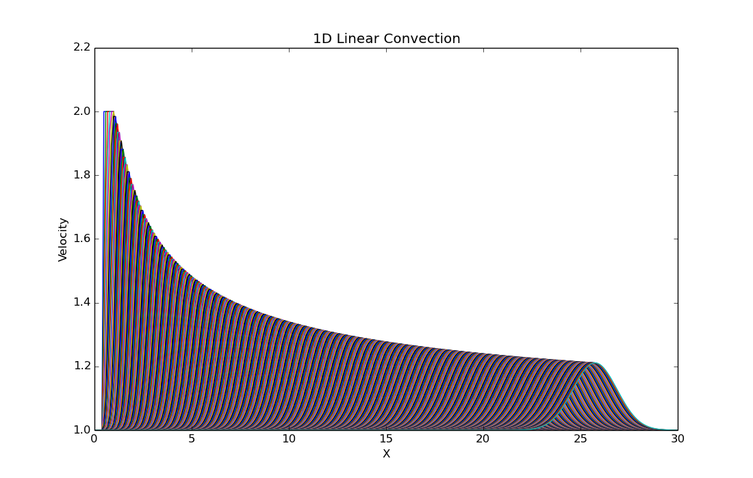
Plotting all steps on the same graph we can see the evolution of the wave profile.

It is clear that the wave is traveling to the positive direction, with no change in shape; the high of the wave is decreasing until solution reaches convergence.

With the values $D=30$, $T=25$, $nx=301$, $nt=500$,we obtain the solution plotted below ($500$ iterations); this shows that the amplitude of the wave will slowly decay until it would reach the value of $1$.