1D Nonlinear Convection

1D Nonlinear convection equation is similar with the linear convection; the change is that the wave is not moving at a constant speed of $c=1$ , but with the speed $u$ :

${\partial u \over \partial t} + u \cdot {\partial u \over \partial x} = 0$

This makes the equation non-linear and more difficult to solve; the differential equation is approximated in the following way:

${u^{n+1}_i - u^n_i \over \Delta t} - u^n_i \cdot {u^n_i-u^n_{i-1} \over \Delta x} = 0$

After separating the unknown $u^{n+1}_i$ , the finite deference scheme is the following:

$u^{n+1}_i = u^n_i - u^n_i \cdot {\Delta t \over \Delta x} \cdot (u^n_i - u^n_{i-1})$

This is implemented in Python; ICs are similar with those in the previous section. The code is written as follows:

# Step2: Nonlinear Convection
# in this step the convection term of the NS equations
# is solved in 1D
# this time the wave velocity is nonlinear as in the in NS equations

import numpy as np
import pylab as pl
pl.ion() # all functions will be ploted in the same graph 
# (similar to Matlab hold on)

D = 4.0 # length of the 1D domain
T = 2.0 # total amount of time for the analysis

nx = 201 # number of grid points
dx = D/(nx-1) # distance between any pair of adjacent grid points
grid = np.linspace(0,D,nx) # creating the space grid

nt = 400 # number of time iterations
dt = T/nt # duration of each timestep

u = np.ones(nx) # initializing the matrix for velocities
u[0.5/dx:1/dx+1] = 2.0 # input of initial conditions, same as step1

un = np.ones(nx)
# used only to initialize a matrix with the same dimension as u
# in here will be kept the velocity for current time step

pl.figure(figsize = (11,7), dpi = 100)
for n in range(nt): # loop for time iteration
    un = u.copy() # copy the current time step velocity
    for i in range(1,nx): # loop over the entire space domain
        u[i] = un[i] - un[i]*dt/dx*(un[i]-un[i-1])
        # compute the velocity for
        # this step for the entire grid based on the velocities 
        # in previous time step and grid points
    pl.plot(grid,u) # plots all profiles on the same graph
    pl.ylim([1.,2.2])
    pl.xlabel('X')
    pl.ylabel('Velocity')    
    pl.title('1D Nonlinear Convection')


# Discussion:
# the wave has moved to the right, with a change in shape
# in the same time, the hight is decreased
# increasing the total time will make the scheme unstable if
# there are not enough timesteps
# that is if the time step is increased the problem loose resolution

# as a good recomendation, the time step dt must be corelated with
# the element size, dx
# if the size of element, dx is decreased, so should be the timestep
# the time step should be smaller than the time needed for the wave
# to pass one grid cell
# for this case, the max velocity is 2
# therefore the time step should be less
# than half of the grid cell size
# dt<dx/vmax

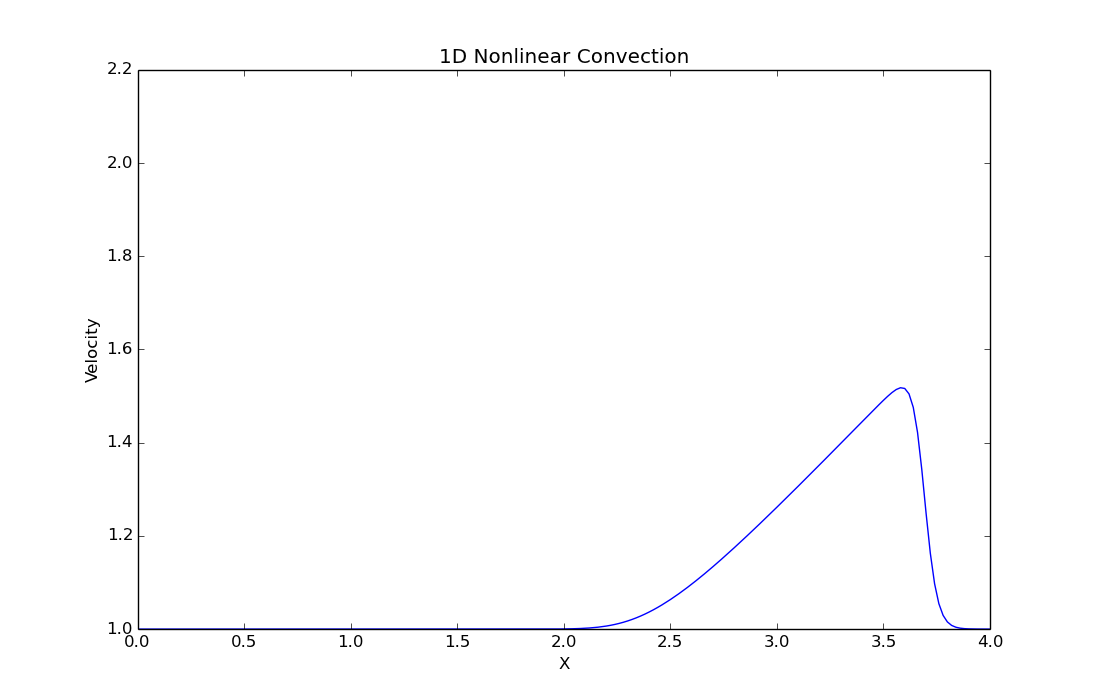
The solution after $400$ iteration is the following:

Plotting all $400$ steps on the same graph we get the following:

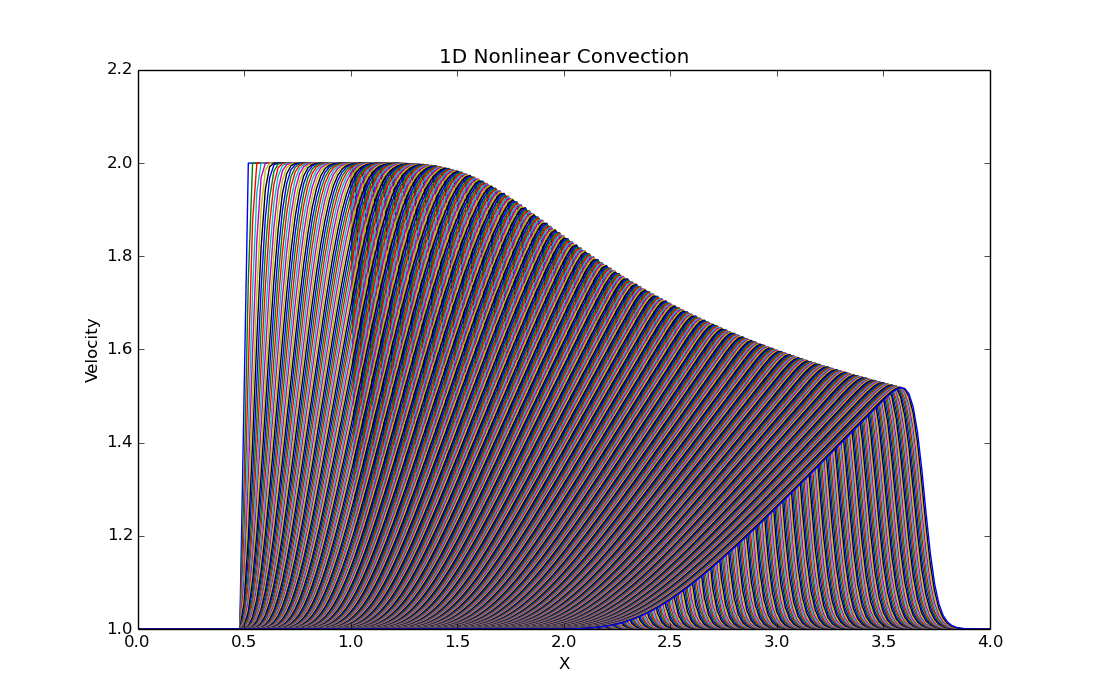
Comparing the solution with that from the linear convection, the following observations can be made:

the wave has moved to the right, with a change in shape;
in the same time, the height is decreased (similar to linear);
increasing the total time will make the scheme unstable if there are not enough time-steps; that is if the time step is increased the problem loose resolution;
as a good practice, the time step dt must be correlated with the element size, dx; if the size of element, dx is decreased, so should be the time-step;
the time step should be smaller than the time needed for the wave to pass one grid cell; for this case, the max velocity is 2, therefore the time step should be less than half of the grid cell size: dt<dx/vmax.

In the next section we will be solving the 1D Diffusion component from the Navier Stokes equation.