Steady turbulent flow over a backward-facing step

In this example we shall investigate steady turbulent flow over a backward-facing step. The problem description is taken from one used by Pitz and Daily in an experimental investigation.

Problem description

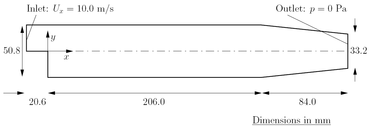
The domain is 2 dimensional, consisting of a short inlet, a backward-facing step and converging nozzle at outlet.

Governing equations:

• Mass continuity for incompressible flow

$${\partial u \over \partial x} + {\partial v \over \partial y} + {\partial w \over \partial z} = 0$$

• Steady state flow momentum equation

$$\nabla (U \bullet U) - \nabla(\nu_{eff} \nabla U) = - \nabla p$$

Initial conditions: $U = 0 m/s, p = 0 Pa$.

Boundary conditions:

• Inlet (left) with fixed velocity $U = (10, 0, 0) \ m/s$;
• Outlet (right) with fixed pressure $p = 0 \ Pa$;
• No-slip walls on other boundaries.

Transport properties: kinematic viscosity of air $\nu = {\mu / \rho} = 18.1 \cdot 10^{−6}/1.293 = 14.0 \ \mu m^2/s$

Turbulence model:

• Standard $k - \epsilon$;
• Coefficients: $C_{\mu} = 0.09$, $C_1 = 1.44$, $C_2 = 1.92$, $\alpha_k = 1$, $\alpha_{\epsilon} = 0.76923$.

Solver name: simpleFoam.

Mesh generation

The domain is subdivided into 12 blocks:

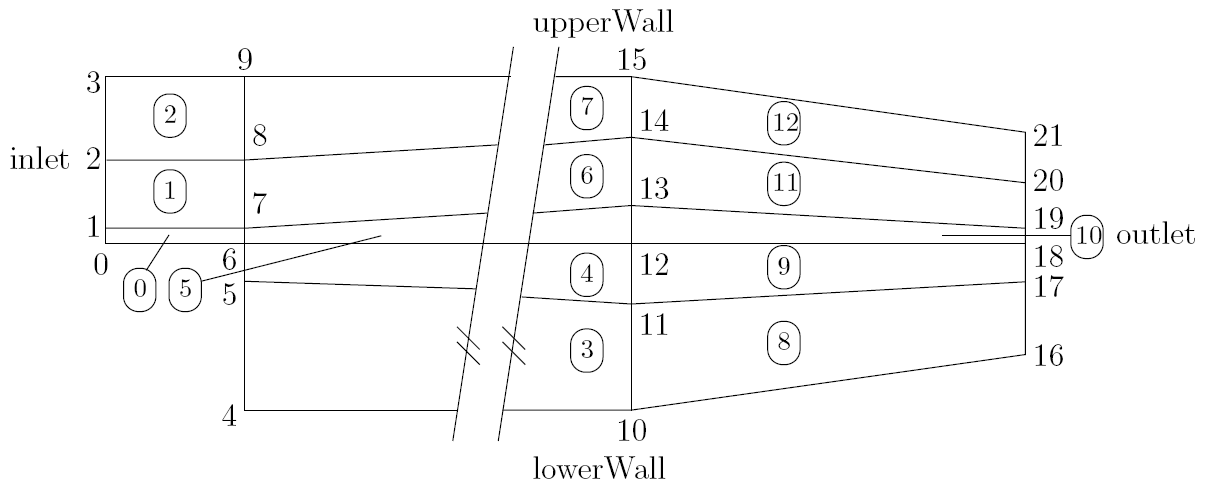
The resulting mesh is the following:

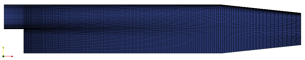
In general, the regions of highest shear are particularly critical, requiring a finer mesh than in the regions of low shear. We can anticipate that high shear will occur close to the center-line of the domain and close to the walls; as it can be seen we have finer cells in these areas.

Boundary conditions and initial fields

We set the initial and boundary fields for velocity $U$, pressure $p$, turbulent kinetic energy $k$ and dissipation rate $\epsilon$. $U$ is given in the problem specification, but the values of $k$ and $\epsilon$ must be chosen by the user.

Assuming that the inlet turbulence is isotropic and the fluctuations are $5 \%$ of $U$ at the inlet, we have:

$$U'_x=U'_y=U'_z={5 \over 100} \cdot 10 = 0.5 \ m/s$$

$$k = {3 \over 2} \cdot (U')^2 = 0.375 \ m^2/s^2$$

With a turbulent length scale of $10 \%$ of the width of the inlet, we can compute the dissipation rate as:

$$\epsilon = {C^{0.75}_\mu \cdot k^{1.5} \over l} = 14.855 \ m^2/s^3$$

At the outlet we need only specify the pressure $p = 0 \ Pa$.

Case control

The problem is incompressible, turbulent and steady state; we will use the solver simpleFoam.

For the steady state analyses relaxation factors apply; a relaxationFactor of $0.7$ is applied for $U$, $k$, $\epsilon$ and $R$; a factor of $0.3$ is required for $p$ to avoid numerical instability.

Results

The solution converged in $765$ iterations; for steady state problems only the final results have physical meaning; therefore in the following all plots are given for the last iteration.

Pressure plot:

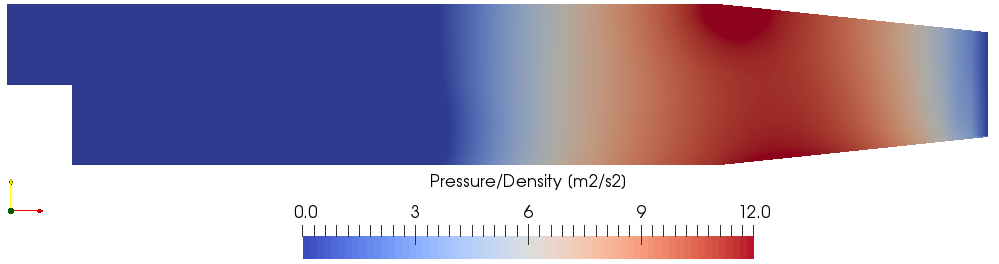
For incompressible problems, OpenFOAM computes the pressure/density as a single variable; the results are valid for any incompressible fluid; to obtain the pressure simply multiply the obtained pressure by the density.

Velocity plot:

Velocity streamlines:

This plot clearly shows the recirculation created after the facing step.

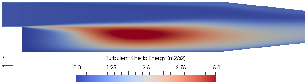
Turbulent kinetic energy plot: